Data Analysis for the Paper

Authors

Affiliations

Elias Bouacida

University Paris 8

Renaud Foucart

Lancaster University

Published

October 7, 2024

Preliminary Data Treatment

The first experiment was run on June 22, July 7 and August 31, 2021, using Amazon Mechanical Turk on a sample of a majority of USA residents. The experiment is hereafter labelled Experiment 1. The second experiment was run on Monday 14, 2023, using Prolific on a representative sample of 600 USA residents. The experiment is hereafter labelled Experiment 2.

We first load the anonymized cleaned data. We have removed from the original output of the data the Prolific and MTURK IDs, that are used for payments. We ensure therefore that the data is anonymous.

First, we load the data from the experiments. We add columns that describe treatments that were not present in the first experiments and align the names of the columns between the different experiments. There was no control for the lottery in the first two AMT experiments.

We load the data from the representative sample, with some renaming to make sure that columns bind together properly afterwards.

We treat age variables to make it consistent between the two experiments.

We bind the data together and simplify the criteria names.

We remove some treatments that we exclude from the analysis. As we have said in the pre-registration, we have removed participants who have not finished the experiment from the data in the cleaning process. We also remove the RPS loser and the arrival time procedures from the first experiment. The latter was formulated differently from the Time treatments later on (the time was not randomly given or chosen, but it was their arrival time).

Section: Experiment 1

Size of the Treatments (Table 1)

In total 1901 participants took part in the experiments.

Table 1: Number of subjects in each experiment

experiment	Number of participants
1	1324
2	577

Table 2: Size of the sample for each treatment.

		Experiment 1		Experiment 2
		Control on the Lottery?
Non-lottery procedure	Control?	No	No	Yes
RPS	No	140	152	-
RPS	Yes	99	98	291
Paintings	No	114	123	-
Paintings	Yes	89	97	-
Time	No	91	106	-
Time	Yes	113	102	286
Note:
When yes for control, subjects chose the sequence used in the procedure.

Earnings

Table 3: Median time spent and earnings in the two experiment.

		Time Spent
Experiment	Hourly Earnings	Min.	Sec.
1	$20.78	4	40.5
2	$18.75	5	11.0
Note:
There was a mistake in the configuration of the Prolific experiment. We show here what they would have earned without this mistake. In reality, the median hourly earnings are $32.75 . The time is the total time spent in Experiment 2 is from entering Prolific to leaving it, whereas it is only the time spent in the oTree part for Experiment 1.

Table 3 shows the median time spent and hourly earnings in both experiments.

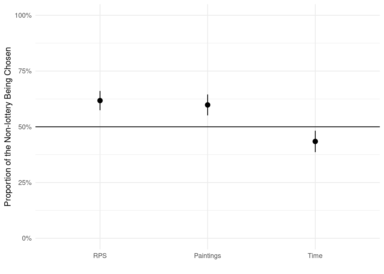
Non-Lottery vs Lottery (Figure 1)

Now we wonder what procedures subjects selected in the different treatments and experiments.

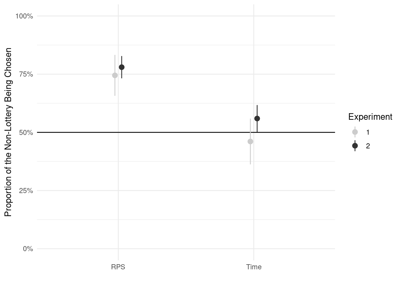
We give in Figure 1 the choices of subjects in Experiment 1, pooling togther all treatments. In Figure 2 we plot on the same results in Experiment 2 and compare them to the corresponding treatments of Experiment 1 (in grey). Table 7 shows that the difference between the two experiments, when in the same treatments, are not significant.

Figure 1: Proportion of each non-lottery procedure being chosen in Experiment 1, pooling treatments with and without control. The error bars represent the 95% confidence interval and the point the estimate for a one sample two-sided t-test of equality with 50%.

We run the first analysis with all subjects.

Table 4: Proportion and P-value of the proportion of the non-random procedure being chosen in each experiment.

Treatment	Experiment	Ritual Chosen	P-value^1^
RPS	1	61.8%	<0.001
Paintings	1	59.8%	<0.001
Time	1	43.4%	0.008
RPS	2	78.0%	<0.001
Time	2	55.9%	0.044
¹ P-value of the one sample two-sided t-test of equality with 50%.

Table 4 shows that in Experiment 1, RPS and Paintings are chosen significantly more than 50% of the time, whereas Time is chosen significantly. In Experiment 2, both RPS and Time are chosen significantly more than 50% of the time.

Table 5: Number of subjects choosing RPS and Time in both experiment, pooling all treatments together, and p-value of the Fisher test of equal proportion between RPS and Time for each experiment.

Experiment	Lottery Chosen	RPS	Time	P-value
1	FALSE	302	179	<0.001
1	TRUE	187	233	<0.001
2	FALSE	227	160	<0.001
2	TRUE	64	126	<0.001

Given the difference in the proportion between the RPS and Time rituals, we can nevertheless test if the proportions are equal or not. Table 5 shows that the proportion are significantly different: our participants chose RPS more often than Time in both experiments.

There is no significant difference in the choice of the non-random procedure comparing RPS and Paintings (the p-value of the Fisher test of the proportion of subjects choosing the non-random procedure being different is ).

Regression Analysis (Table 2)

Table 6: Regression analysis: share of subjects choosing a non-lottery procedure in Experiment 1, where the baseline is RPS with control and Lottery without control.

Regression analysis: share of subjects choosing a non-lottery procedure in Experiment 1, where the baseline is RPS with control and Lottery without control
	Non-Lottery Chosen
	Simple	Controls
(Intercept)	0.695***	0.699***
	(0.032)	(0.078)
Time	-0.190***	-0.191***
	(0.033)	(0.033)
Paintings	-0.028	-0.024
	(0.032)	(0.032)
Win only in Non-Lottery¹	0.114***	0.112***
	(0.033)	(0.033)
Win only in Lottery¹	-0.099**	-0.098**
	(0.035)	(0.035)
No Control on Non-Lottery	-0.053*	-0.050+
	(0.027)	(0.027)
Control on Lottery	-0.103***	-0.107***
	(0.027)	(0.027)
Male		0.052+
		(0.027)
Age Controls²	No	Yes
Num.Obs.	1324	1317
R2	0.059	0.065
R2 Adj.	0.055	0.058
+ p < 0.1, * p < 0.05, p < 0.01, * p < 0.001
¹ Win only in XX is a dummy for when a subjects believe they will win the XX procedure and NOT in the alternative one.
² Age controls: Control for the age categories, none are significant.

Experiment 2 (Figure 2)

In Table 7, we show that in both experiments, the proportion of subjects choosing the non-lottery is significantly above 50% for RPS. For Time, the results differ between the two experiments. The result from Experiment 2, where Time is significantly more chosen that 50%, should be seen as more robust, as it is on a representative sample of the population.

Table 7: Proportion of subjects choosing one procedure over the other in both experiments.

Procedure	Experiment	Proportion	P-value
RPS	1	74.5%	<0.001
RPS	2	78.0%	<0.001
Time	1	46.1%	0.431
Time	2	55.9%	0.044
Note:
P-value of the one sample two-sided t-test of the proportion being equal to 50%.

Table 8: Are the proportions of subjects choosing Time and RPS significantly different between the two experiments (in the same treatments)?

criteria	lottery_chosen	exp1	exp2	fisher_est	fisher_pval
RPS	FALSE	73	227	0.8237051	0.489
RPS	TRUE	25	64	0.8237051	0.489
Time	FALSE	47	160	0.6736616	0.105
Time	TRUE	55	126	0.6736616	0.105

Figure 2: Proportion of each non-lottery procedure being chosen in Experiment 2. Results in experiment 1 are shown in grey, in the same treatment conditions.

We have tried to get at the strength of preferences by asking the willingness to accept for their choice being removed. We find only 3.1% of subjects state indifference in Experiment 2 (by stating a WTA of $0). Table 9 shows that removing indifferent subject from the sample does not change the proportion chosen.

Table 9: Are the proportions in Experiment 2 for choosing Time and RPS different including indifferent subjects and excluding them?

criteria	lottery_chosen	not_strict	strict	fisher_est	fisher_pval
RPS	FALSE	227	217	0.9807328	>0.999
RPS	TRUE	64	60	0.9807328	>0.999
Time	FALSE	160	159	0.9823565	0.933
Time	TRUE	126	123	0.9823565	0.933

Section 4: Robustness

Our Procedures Are Unpredictable (Table 3)

We know assess how well subjects predict their own future performance.

Table 10: Correlation between real and believed performance. P-value of the correlation test are in parenthesis.

Correlation (p-value)
Non random	Lottery
0.006 (0.787)	-0.003 (0.911)

Table 11: Correlation between real and believed performance in each procedure, for both experiments.

Non-lottery	Correlation (p-value)
Procedure	Non-lottery	Lottery
Experiment 1
RPS	0.01 (0.825)	0.035 (0.44)
Paintings	-0.031 (0.522)	-0.013 (0.783)
Time	-0.047 (0.344)	0.033 (0.511)
Experiment 2
RPS	0.11 (0.061)	-0.032 (0.582)
Time	0.036 (0.545)	-0.071 (0.234)
Note:
P-value of the correlation test of the correlation being equal to 0 in parenthesis.

Rock, paper, scissors

We look at the choices in RPS, to check for the bias in favour or Rock.

Table 12: Choices in Rock, Paper, Scissors.

Overall			In the first round
Rock	Paper	Scissors	Rock	Paper	Scissors
37.5%	34.8%	27.7%	44.7%	35.6%	19.6%

Beliefs and Overconfidence (Table 4)

Table 13 shows some overall overconfidence, as more than 50% of subjects believe they will win in either the criteria or the lottery. To see if beliefs influence choices, we can look at the subjects who believe they will win in the criteria but not in the lottery and the reverse. If beliefs are the only driver of choices, then the first group should always choose the criteria, and the second group should always choose the lottery. Table 16 shows that it is not the case. P-value of the Fisher test shows that beliefs have only a minor influence as well.

Table 13: Percentage of subjects who believe they will win in the lottery or the criteria.

Experiment	Treatment	Winning in non-Lottert	Winning in Lottery
RPS	1	60.7%	59.5%
Paintings	1	65.5%	58.6%
Time	1	58.3%	55.8%
RPS	2	72.5%	56.0%
Time	2	62.9%	53.5%

Table 14: Overall overconfidence: do subjects believe they will win in the non-lottery more than in the lottery procedures?

Experiment	Non-Lottery Procedure	Belief	Non-Lottery	Lottery	P-value<sup>1</sup>
1	RPS	Win	297	291	0.744
1	RPS	Loose	192	198	0.744
1	Paintings	Win	277	248	0.047
1	Paintings	Loose	146	175	0.047
1	Time	Win	240	230	0.527
1	Time	Loose	172	182	0.527
2	RPS	Win	211	163	<0.001
2	RPS	Loose	80	128	<0.001
2	Time	Win	180	153	0.027
2	Time	Loose	106	133	0.027
¹ P-value of the Fisher exact test of the proportion of subjects stating that they will win in one procedure (non-lottery or lottery) being the same.

Table 15: Proportion of subjects saying that they will win in a procedure.

		Control		Belief Win in
Experiment	Procedure	Non-random	Lottery	Non-random	Lottery	P-value<sup>1</sup>
1	RPS	FALSE	FALSE	64.5%	59.2%	0.347
1	RPS	FALSE	TRUE	62.9%	60.7%	0.713
1	RPS	TRUE	FALSE	53.1%	56.1%	0.669
1	RPS	TRUE	TRUE	59.6%	61.6%	0.773
1	Paintings	FALSE	FALSE	71.5%	64.2%	0.221
1	Paintings	FALSE	TRUE	56.1%	60.5%	0.504
1	Paintings	TRUE	FALSE	64.9%	50.5%	0.042
1	Paintings	TRUE	TRUE	69.7%	57.3%	0.088
1	Time	FALSE	FALSE	55.7%	49.1%	0.338
1	Time	FALSE	TRUE	50.5%	42.9%	0.301
1	Time	TRUE	FALSE	65.7%	69.6%	0.552
1	Time	TRUE	TRUE	60.2%	60.2%	>0.999
2	RPS	TRUE	FALSE	72.5%	56.0%	<0.001
2	Time	TRUE	FALSE	62.9%	53.5%	0.022
¹ P-value of the two-sided two-sample t-test of the proportion between the non-lottery procedure and the lottery being the same.

Table 16: Percentage of subjects who choose the non-lottery conditional on their beliefs of winning in the non-lottery but not the lottery and the reverse. P-value of the proportions being the same.

	Subjects expect to win only in
Non-lottery Procedure	Non-Lottery	Lottery	P-value^1^
Experiment 1
RPS	79.1%	46.2%	<0.001
Paintings	67.0%	43.7%	0.003
Time	50.6%	45.3%	0.530
Experiment 2
RPS	84.9%	63.2%	0.010
Time	63.8%	45.2%	0.117
Note:
The first column represents subjects expecting to win in the non-lottery procedure but not in the lottery, the second column the reverse.
¹ P-value of the Fisher test of the proportions of subjects who believe they will win in one procedure but not the other who choose the non-lottery procedure being equal.

Table 17: Percentage of subjects who choose the criteria conditional on their beliefs of winning in criteria but not the lottery and the reverse, in Experiment 2 when preferences are strict. P-value of the proportions being the same.

	Subjects expect to win only in
Non-Lottery Procedure	Non-Lottery	Lottery	P-value^1^
RPS	85.4%	66.7%	0.026
Time	63.2%	45.2%	0.120
Note:
The first column represents subjects expecting to win in the non-lottery procedure but not in the lottery, the second column the reverse.
¹ P-value of the Fisher test of the proportions of subjects who believe they will win in one procedure but not the other who choose the non-lottery procedure being equal.

Appendix

Appendix A Experiment 1 (Table 5)

Table 18: Proportion of subjects choosing a procedure if they have control or no control on the lottery in Experiment 1.

	Chosen Procedure
	Number		Proportion		P-value
Control	Lottery	Non-lottery	Lottery	Non-lottery	P-value
FALSE	267	411	39.4%	60.6%	<0.001
TRUE	323	323	50.0%	50.0%	<0.001
Note:
P-value of the Fisher exact test of equal proportions.

Table 19: Proportion of subjects choosing a procedure with and without control on the non-lottery procedure in Experiment 1.

	Chosen Procedure
	Number		Proportion		P-value
Control	Lottery	Non-Lottery	Lottery	Non-Lottery	P-value
FALSE	334	392	46.0%	54.0%	0.267
TRUE	256	342	42.8%	57.2%	0.267
Note:
P-value of the Fisher exact test of equal proportions.

Table 20: Proportion of subjects choosing a procedure if they have control or no control on the non-random procedure in Experiment 1.

		Chosen Procedure
		Number		Proportion
Non-lottery Procedure	Control	Lottery	Non-lottery	Lottery	Non-lottery	P-value<sup>1</sup>
Rituals	FALSE	222	307	42.0%	58.0%	0.046
Rituals	TRUE	135	248	35.2%	64.8%	0.046
Time	FALSE	112	85	56.9%	43.1%	0.921
Time	TRUE	121	94	56.3%	43.7%	0.921
Note:
Rituals group together the RPS and Time procedures.
¹ P-value of the Fisher exact test of equal proportions.

Table 21: Proportion of subjects choosing the non-lottery procedure in Experiment 1, for each treatment.


Control in
Non-Lottery	Yes	Yes	No	No
Lottery	No	Yes	No	Yes
Non-lottery procedure
RPS	74.5%	58.6%	65.1%	51.4%
Paintings	66.0%	59.6%	62.6%	51.8%
Time	46.1%	41.6%	48.1%	37.4%
Note:
Share over all subjects in their respective sample.

Appendix B Experiment 2 (Table 6)

Table 22: Share of subject choosing the non-lottery procedure in Experiment 2. The baseline is RPS (with control).

Share of subject choosing the non-lottery procedure in Experiment 2. The baseline is RPS (with control).
	Non-Lottery Chosen
	Simple	Controls
(Intercept)	0.780***	0.848***
	(0.032)	(0.070)
Time	-0.221***	-0.223***
	(0.038)	(0.038)
Win only in Non-Lottery¹	0.077+	0.076+
	(0.045)	(0.046)
Win only in Lottery¹	-0.126*	-0.132*
	(0.060)	(0.060)
Indifferent	-0.127	-0.120
	(0.109)	(0.110)
Male		-0.044
		(0.038)
Demographic Controls²	No	Yes
Num.Obs.	577	577
R2	0.073	0.079
R2 Adj.	0.066	0.064
+ p < 0.1, * p < 0.05, p < 0.01, * p < 0.001
¹ Win only in XX is a dummy for when a subjects believe they win the XX procedure and NOT in the alternative one.
² Demographic controls: Age categories, Being White, No demographic control was significant.

Appendix C (Table 7)

Table 23: Correlation between real and believed performance, taking into account control. P-value of the correlation test are in parenthesis.

Non-lottery	Control on		Correlation (p-value)
Procedure	Non-lottery	Lottery	Non-lottery	Lottery
Experiment 1
RPS	No	No	0.11 (0.177)	-0.027 (0.743)
RPS	No	Yes	-0.118 (0.164)	0.161 (0.058)
RPS	Yes	No	-0.041 (0.689)	-0.021 (0.841)
RPS	Yes	Yes	0.091 (0.372)	0.008 (0.938)
Paintings	No	No	0.023 (0.799)	-0.016 (0.863)
Paintings	No	Yes	-0.197 (0.036)	-0.033 (0.726)
Paintings	Yes	No	0.18 (0.077)	0.031 (0.766)
Paintings	Yes	Yes	-0.115 (0.284)	-0.036 (0.74)
Time	No	No	-0.066 (0.505)	0.018 (0.856)
Time	No	Yes	0.01 (0.924)	-0.089 (0.401)
Time	Yes	No	-0.185 (0.063)	0.159 (0.111)
Time	Yes	Yes	0.033 (0.731)	0.033 (0.731)
Experiment 2
RPS	Yes	No	0.11 (0.061)	-0.032 (0.582)
Time	Yes	No	0.036 (0.545)	-0.071 (0.234)
Note:
In parentheses are the p-value of the correlation test of the correlation being different from 0.

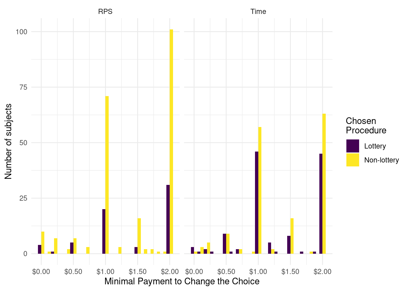
Appendix D Intensity (Table 8 and Figure 3)

We classify subjects according to their WTA to change their choices in Table 24.

Table 24: Number of subjects and strength of their preference.

Non-lottery Procedure	Procedure Chosen	Indifferent	Strict Preferences
RPS	Lottery	4	60
RPS	RPS	10	217
Time	Lottery	3	123
Time	Time	1	159
Note:
A preference is considered strict if the WTA is non-null.

Figure 3: Minimum amount we would need to pay subjects for them to change their choice. Remember that the reward given by the procedure is $2.

Appendix E: Demographics (Table 9-12)

43.0% of participants in the sample are female. Table 26 shows the repartition of the different age groups in both experiments. Table 27 shows a the repartition of ethnicity using Prolific stratification strategy.

Table 25: Self-declared gender balance of the sample in each experiment.

Gender	Experiment 1	Experiment 2
Female	38.8%	52.5%
Male	61.2%	47.5%

Table 26: Proportion of subjects in each age group for each experiment.

Age Group	Experiment 1	Experiment 2
<25	3.5%	13.9%
25-40	64.6%	28.9%
40-55	23.2%	25.8%
>55	8.2%	31.4%
Prefer not to say	0.5%	-

Table 27: Declared ethnicity in Experiment 2.

Declared Race	Count
Asian	36
Black	76
Mixed	12
Other	6
White	447

Table 28: Country of residence of participants in the experiments.

Country	Experiment 1<sup>1</sup>	Experiment 2
Asian	0.2%	-
Brazil	4.2%	-
Bulgaria	0.1%	-
Canada	0.5%	-
Columbia	0.1%	-
France	0.3%	-
Germany	0.3%	-
India	12.2%	-
Italy	1.5%	-
Portugal	0.1%	-
Spain	0.2%	-
Sweden	0.1%	-
The Netherlands	0.1%	-
Turkey	0.1%	-
UAE	0.2%	-
USA	79.3%	100.0%
Ukraine	0.1%	-
United Kingdom	0.5%	-
¹ In Experiment 1, the country is residence is self-declared. We reconstructed the intended country as best as we could.

Appendix F: Choice Sequence (Tables 13-14)

It is possible that participants are influenced in their choices by the strategies we choose for then when they have no control over a procedure. As a reminder, TRUE (aka 1) is even, while FALSE (aka 0) is odd (which is an odd choice we made).

Table 29: Choices of the non-lottery procedure when subjects have no control over the lottery, by the number of Even in the sequence given to them.

	Number of evens						P-values
	0	1	2	3	4	5	0~5	1~4	2~3
Experiment 1
RPS	40.0%	63.6%	65.0%	77.5%	76.9%	50.0%	>0.999	0.234	0.108
Paintings	66.7%	63.4%	70.0%	62.2%	52.2%	75.0%	>0.999	0.433	0.375
Time	28.6%	39.3%	49.2%	54.3%	34.4%	62.5%	0.315	0.791	0.604
Experiment 2
RPS	88.9%	86.5%	78.6%	78.3%	71.9%	60.0%	0.505	0.139	>0.999
Time	37.5%	53.2%	60.4%	51.7%	56.5%	85.7%	0.119	0.836	0.290
Aggregate	52.5%	61.9%	65.1%	64.9%	61.3%	67.6%	0.237	0.918	>0.999
Note:
P-values of the Fisher exact test of equal proportion in both samples.

We establish before that the number of even or odd in the sequence do not significantly influence the choice of the non-random procedure or the lottery. Now we group together even and odds.

Table 30: Choices of the non-lottery procedure when subjects have no control over the lottery, by the number of Even/odd in the sequence given to them.

	Number of evens/odds			P-values
Non-lottery procedure	0	1	2	0~1	0~2	1~2
Experiment 1
RPS	43.8%	69.9%	70.9%	0.081	0.045	0.882
Paintings	71.4%	59.4%	65.5%	0.548	0.773	0.436
Time	46.7%	36.7%	51.9%	0.558	0.789	0.062
Experiment 2
RPS	78.6%	77.2%	78.4%	>0.999	>0.999	0.881
Time	60.0%	54.8%	56.2%	0.785	>0.999	0.898
Aggregate	59.5%	61.6%	65.0%	0.795	0.374	0.251
Note:
P-values of the Fisher exact test of equal proportion for each procedure between each number of sequence.